
About
Hi, I am Daniele and I am a Mathematical Engineer. I work as an Applied Scientist at Zalando, specifically optimizing logistics and supply chain.
I have a Ph.D. in pure and applied mathematics at Politecnico di Torino. The application context was decision-making under uncertainty in engineering/management applications.Practically speaking, someone pays me to generate wrong models of real problems. However, this is what people call engineering, and unexpectedly, it (may) work too. I also do some data science, developing structured ad-hoc solutions more than very general approaches.I earned my Master's degree in mathematical engineering at Politecnico di Torino and Technische Universiteit Eindhoven summa cum laude. During my Master's, I was a post-graduate research assistant for the development of software for the generation of a polyhedric mesh in domains with randomly generated interfaces for F.E.M. (better be convex). I also worked as a visiting researcher at the Technical University of Munich for a collaborative research project in the area of multi-echelon perishable inventory management at the logistics and supply chain management department.After my PhD, I worked as research scientist for two years at the German Aerospace Center (DLR) in the Institute for the Protection of Terrestrial Infrastructures. Mainly, I developed models for adaptive mission planning of autonomous unmanned systems during dynamic environmental hazards and designed mathematical programming approaches for evacuation planning during disasters. I also contributed to smaller projects, such as hospital timetabling and machine learning models for predicting failures in critical infrastructures.Besides doing math, I play the trumpet (still trying to play the IV Arban's Carnival of Venice variation with no errors) and do fitness (I once got a fitness trainer certificate, but nothing serious, I was curious). A long time ago, I also earned a pre-academic certification in trumpet at the Superior Institute of Musical Studies of Caltanissetta.This website serves as a general presentation of myself and as a record of my posthumous thoughts on my academic works.
Recent News
With my team MathConvoy, we placed second at the INFORMS RAS 2025 Problem Solving Competition at the 2025 INFORMS annual meeting. Specifically, using operations research and advanced analytical approaches, we created a predictive maintenance tool for rail systems. Using wheel profile data, mileage, railcar attributes and other sensor measurements, the tool predicts wheel failures on commercial trains.
The paper Sequential Drone Routing for Data Assimilation on a 2D Airborne Contaminant Dispersion Problem, presented at the 16th IEEE Symposium Sensor Data Fusion has won the best paper award. Navier–Stokes viscosity was like honey, but the sequential policy was nice :).
With my team Scienza Sabauda we won the Data-Driven Logistics and Supply Chain Competition organized by SCAIL, University of Cambridge (Supply Chain AI Lab) as the most innovative solution at the 18th IFAC Symposium on Information Control Problems in Manufacturing (INCOM 2024). At the same conference, we were nominated as best paper award finalist with the work Joint Discount and Replenishment Parametric Policies for Perishable Products_.
Working_On
Most of my applications so far require making sequential decisions under uncertainty. A diverse array of problems addressed during my academic journey is presented hereafter. Tools employed to provide decision aid include stochastic programming, dynamic programming, Bayesian metamodels, and simulation-based optimization. For a better understanding of the paradigms governing sequential decisions under conditions of uncertainty, I suggest the work of Warren Powell and Dimitri Bertsekas, who have devoted a large part of their career to this topic.Everything you read here has, by its very nature, already been superseded; through a more accurate understanding, a needed correction, a more suitable method, or a consequent extension thereof.
Data assimilation and adaptive routing
Environmental emergency scenarios often involve dynamic hazards whose progression is difficult to predict due to inherent uncertainties and time dependencies. Although mathematical models exist to approximate these dynamics, they are often incomplete or imprecise. Consequently, real-time data are crucial for refining understanding of the situation, enhancing situation awareness and improving response strategies.
Recent advances in autonomous unmanned systems, such as drones or tracked robots, have enabled rapid, on-the-ground data collection.
In the article A perspective and review on adaptive mission planning and hazard monitoring during emergencies with autonomous unmanned systems, published in Annual Reviews in Control, I provide a perspective and structured synthesis of techniques for integrating in situ observations into adaptive models for situation awareness, framed through an overarching sequential decision-making view and a control hierarchy for autonomous unmanned systems.I have also been developing some preliminary data assimilation solutions where an ensemble Kalman filter is used to sequentially exploit and improve an advection-diffusion model numerically solved by FEM of an airborne contaminant dispersion problem over a chemical plant. An autonomous observer is routed according to the available knowledge at each decision time with a simple but interesting policy; sequentially observing the contaminant concentration in a small fraction of the non-simply connected domain. Such observations are synchronized with the data assimilation framework, iteratively adapting the simulation.
A pre-print of a contribution presented at the 16th Symposium Sensor Data Fusion is available on ArXiv, winner of the best paper award.

Inventory control of perishable items

The new sustainable development goals are considered a blueprint to achieve a better and more sustainable future for all. Reduction of losses and overstocking on supply chains and retail environments are central topics, even more so when the considered items have a short life (i.e. food, blood platelets). I tried to deal with advanced inventory management control systems that employ different mathematical methods. However parametrical policies seem to be the most accepted in this domain.A study that allows for a multi-item setting with substitution between similar goods, deterministic deterioration, delivery lead times, and seasonality was presented in Nantes at the 10th IFAC Conference on Manufacturing Modelling, Management and Control MIM, with the title Inventory management of vertically differentiated perishable products with stock-out based substitution. This work was extended and presented in more detail and comprehensively in Computer & Operation Research, in the article Simulation-based inventory management of perishable products via linear discrete choice models. An open-source simulation-based framework has been developed, filling the lack of open-source libraries in the perishable inventory literature, and released on GitHub.
Given their dimensional complexity and the strong autocorrelation within each simulated process, the best numerical strategy to optimize the policies I investigated is still an open problem and not solved in the article.
An extension of the model that deals with discount policies and orders in batches has been presented at the 18th IFAC Symposium on Information Control Problems in Manufacturing, where it was a finalist for the best paper award. The title is Joint Discount and Replenishment Parametric Policies for Perishable Products.Another work on perishable items, dealing with Multichannel and omnichannel multi-echelon networks is published in Transportation Research Part E: Logistics and Transportation Review with the title On the value of multi-echelon inventory management strategies for perishable items with on-/off-line channels. There, a dynamic model is proposed, jointly optimizing allocation and replenishment policies in the case of perishable goods with stochastic demand, uncertainty in customer selection preferences, and fixed lead times on online/offline channels. In short, I tried to generalize base-stock policies over multi-echelon networks, analyzing the effect that potential correlations and imbalances in demand volumes across channels generate on the heuristics. The correspondent library is available on GitHub.All these works suffer from two major unresolved complexities: 1) flexible and accurate convergence management for each evaluated simulation 2) the choice of an optimizer that understands the structure of the problem.
Assemble-to-Order Problems
Assemble-to-order is a production strategy where components are manufactured under demand uncertainty and end items are assembled only after demand is realized. This strategy is commonly applied to hedge against significant uncertainties in the order of the end items, naturally leading to Two-Stage and Multi-Stage Stochastic Programming formulations. I applied some ad-hoc reinforcement learning strategies to reduce the Multi-Stage complexity and study different multistage multi-item models, showing how they behave, based on the usage of the available information.
An article that deals with seasonality, bimodality, and correlations in the distribution of end items demand, where the approximation of terminal values and rolling horizon simulations are applied has been published in the International Journal of Production Research, with the title Rolling horizon policies for multi-stage stochastic assemble-to-order problems. A preprint version is available on ArXiv. The code is open-source and available on GitHub.
A book chapter contribution that tackles these problems with risk-averse models in a two-stage stochastic linear programming setup, considering the introduction of a classical risk measure from finance is available in
Optimization and Decision Science: Operations Research, Inclusion and Equity, part of AIRO Springer Series.

Control and design optimization of Wave Energy Converters
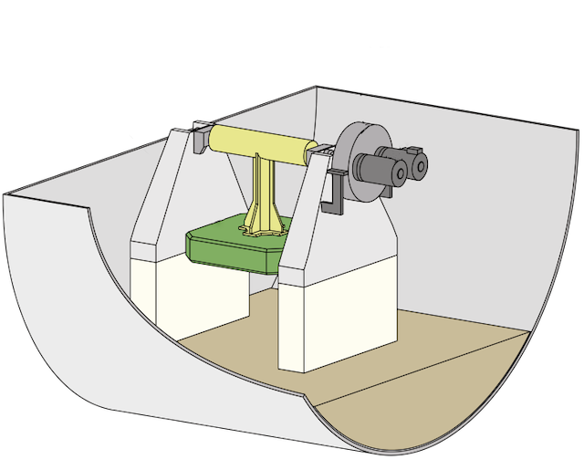
The energy problem related to the pursuit of alternatives to fossil fuels is an active challenge for the entire world. Unlike other types of energy conversion technologies, such as photovoltaic plants or wind turbines, wave energy converters (WECs) have not reached a sufficient level of technological maturity and two of the most crucial issues are: the development of suitable advanced control strategies for WEC devices and the optimal design in terms of cost and extracted energy.
I tried to develop some strategies that apply a Gaussian Process Regression (GPR) optimization approach to compute the parameter of a reactive control action in the article: Data-driven control of a Pendulum Wave Energy Converter: A Gaussian Process Regression approach, published by Ocean Engineering. Although it is not my domain, I also lent a hand on techniques to robustify the physical design against mechanical mismatches, co-authoring the conference proceedings Wave Energy Converter Optimal Design Under Parameter Uncertainty presented at the ASME 2022 41st International Conference on Ocean, Offshore and Arctic Engineering.
Other works
One of the first things I worked on in 2020 during my Master's thesis involved optimizing long-term portfolios. In general, however, I moved FAR away from such applications. Main reason being the posthumous understanding of fat tails.
The few ideas I had about it were about the building of very general decision support systems able to make usable whatever performance and risk metric the decision-maker considers adequate (e.g., deep learning strategies), allowing for known instruments like technical and fundamental analysis, and attempting to overcome some of the inherent complexities and limitations of the most classical and practically useless strategy: Markowitz's. An academic article titled Early portfolio pruning: a scalable approach to hybrid portfolio selection has been published in Knowledge and Information Systems by Springer Nature. There, a hybrid approach that combines itemset extraction and Markowitz’s model logic, generalizing the idea of balancing profit and risk, but dealing with sets of candidate portfolios rather than with single stocks and allowing for technicals, fundamentals and risk measures. This paper presents experiments that validate the strategy by using back-testing. However, back-testing is FULL of biases, which I discuss in the technical notes of this website. The contribution is therefore more methodological than pragmatic.

Reviews
An integral part of research work, often unrecognized, involves reviewing and contributing to the work of others. This is done anonymously and for free. However, it costs days and days. Besides conferences, to date, I have given reviews of various articles for:-European Journal of Operations Research
-Computer & Operations Research
-International Journal of Production Economics
-Applied Mathematical Modelling
-Journal of Retailing and Consumer Services
-International Transactions in Operational Research
-Computers and Industrial Engineering
-RAIRO - Operations Research
(Very) Technical_Notes
Despite authors' and reviewers' efforts, most academic articles naturally contain typos and some (hopefully small) necessary posthumous corrections. I do have typos and errors in my works and I collected (the ones I know) here.In general, research is dynamic. Unfortunately, or fortunately, experience requires time.
Daniele Giovanni Gioia, Leonardo Kanashiro Felizardo, and Paolo Brandimarte. Simulation-based inventory management of perishable products via linear discrete choice models. Computers & Operations Research, page 106270, 2023.
doi:10.1016/j.cor.2023.106270.
Note/Better Formalization: In the practical implementation of dynamic problems, memory cells of a vector are often reused with different meanings during a simulation. However, to make the theoretical exposition clearer, the correct notation for Eqs. (10) and (12) would require that the shelf life indices do not consider the maximum value (being empty because at the end of the day) and that the lead time index iterates semantic values and not memory locations of the vector. In short, the ranges of the sums are best written as:
Typo: At the end of page 5, regarding policies where one item is seasonally managed and the other ones are not, a -1 is missing. The correct dimension is:
Note: The characteristics of the problem directly affect the convergence of the simulated expected value. Use simulations long enough (and repeat)! I also stress that the optimization solver choice is a complex matter. The problem here has a lot of dimensions, with many local optima.
Daniele Giovanni Gioia, Edoardo Pasta, Paolo Brandimarte, and Giuliana Mattiazzo. Data-driven control of a pendulum wave energy converter: A Gaussian process regression approach. Ocean Engineering, 253:111191, 2022. doi:10.1016/j.oceaneng.2022.111191.
Notational clarification: In a consistent way with its use in the rest of the article, In Table 2, and after Eq. (30), lambda represents the variance and not the standard deviation. Furthermore, equation (30) itself does not need a squared lambda.
Notational clarification: After Eq. (32), the kernel operator vector/matrix has an image with dimensionality n, not d. I.e.,
Notational clarification: In Eq.(42) some parenthesis are missing. The correlation coefficient multiplies the noise matrices as well, being:
Daniele Giovanni Gioia and Stefan Minner. On the value of multi-echelon inventory management strategies for perishable items with on-/off-line channels. Transportation Research Part E: Logistics and Transportation Review, 180:103354, 2023.
doi:10.1016/j.tre.2023.103354.
Additional note: In equation 10 there is a slight abuse of notation. In fact, in its practical application, the reward is calculated in two time frames. The part relating to sales before the time shift, while the part relating to salvage values or disposal costs, at the time of scrapping. This means that the inventory with superscript 0 represents the inventory with superscript 1 from which sales are subtracted.
Precision on Table 5 and 6: The max-min width of 0.02% over the 35-period sliding window on the moving window during the learning in the numerical simulations related to the heuristic approaches (Section 4.2) in the article "On the value of multi-echelon inventory management strategies for perishable items with on-/off-line channels" is not achieved. The stopping criterion for the difference between the minimum and maximum values of the statistic associated with the expected value was blocked by a limit on the maximum number of simulated steps (1400), which is insufficient to deal with a width of 0.02%. To asses the effect on the experiments, they were repeated with a maximum number of steps ten times larger, equal to 14000, using the stopping criterion at 0.02% and the optimization strategy presented in Gioia and Minner (2023). For the out-of-sample evaluation, we increase the 7000-period-long horizon five-fold to 35000. Evaluation and optimization of the full design of experiments are here presented in an updated version of Tables 5 and 6 from Gioia and Minner (2023). In general, this heuristic is bad and I should have done something that considers the autocorrelation of the process better. I am sorry for this. At least, Welch's method should be used! Conclusions and remarks in Gioia and Minner (2023) remain valid, but some values have changed slightly. For example, the waste reduction of the BSP policy for a 5-period shelf-life compared to the COP policy has decreased, while the profit values of many multi-echelon policies have improved, as they are more prone to non-convergence of the expected value estimate due to more complex dynamics during simulation than single-echelon policies. It is also reasonable to point out that the very choice of optimization algorithm is practically a hyperparameter of the study and that, using non-surrogate techniques, different results might be obtained.
Additional note: The range of values for the coefficient of variation, if directly modeled by considering an adjusted independent daily adaptation of the weekly estimated values from Broekmeulen and van Donselaar (2019), would be:
However, we deal with products with high daily sales (and low shelf life) and they state and report that under these assumptions perishables are correlated to higher correspondent daily standard deviations. Unfortunately, for confidentiality reasons, they normalize their data and provide only aggregated statistics, making more specific deductions complex. To provide meaningful experiments, we assume higher values and investigate more than one option cv = 0.6, 0.9. focusing on the relative differences in their effects rather than absolute behaviors in a specific case study.
Daniele Giovanni Gioia, Jacopo Fior and Luca Cagliero. Early portfolio pruning: a scalable approach to hybrid portfolio selection. Knowledge and Information Systems 65.6 (2023): 2485-2508. doi:10.1007/s10115-023-01832-7.
The first observation is that I would never do that kind of work again, but think it is normal when you gain experience and understand the limitations of what you have done. However, we have to own the good as well as the bad
The bias of back-testing: One of the big problems with back-testing is data acquisition. Especially in the fintech sector, the appearance would suggest that there is all the data you want. In reality, this is false. When you want to leverage data from fundamentals (e.g., balance sheets and income statements), it is a mess. The difficult question is: are the stocks for which detailed data are available the ones that historically then performed the better? Is a survival bias implied in the possibility of acquiring data itself? Sotcks get delisted. Tickers change. Corporations fuse. All back-tested results inherently depend on the data quality. For this reason, my article, like 99 percent of those concerning fintech, should be used only for methodological scientific advancement and not pragmatically taking its validation results as oracles of superior performance. NASDAQ-100 is used only as a reference, but it changes often and old stock data weren't available. The most important comparisons are with all other methods leveraging on the same pool of available stocks. There is a reason why we only compared established funds on the most recent (at the time of writing (2020)) years and we stressed only those being a real scenario example; that is because of backtesting bias. If you had different data you would get different results, but the method would stay. Let's say that if it had made me a billionaire, I wouldn't have shared it with you.